A one-sample t-test in SPSS helps you compare the mean of one sample to a known, expected, or hypothesized value. If you are working with one group and want to know whether its average differs from a benchmark, SPSS makes the process straightforward. This guide focuses only on how to perform a one-sample t-test in SPSS step by step.
If you want a full explanation of what the test means, when to use it, and its assumptions, read our guide on the one-sample t-test explained. However, if you already know how to run the test in SPSS and need help with writing the results in APA, visit our separate guide on how to report one-sample t-test results in APA.
When the One-Sample T-Test is Appropriate
Use the one-sample t-test in SPSS when you want to determine whether the mean of a single sample differs from a known, expected, or hypothesized value. In simple terms, this procedure answers a question like: Is the average in my sample different from this benchmark?
This test is appropriate when:
- You have one sample or one group
- You have one continuous numeric variable
- You want to compare the sample mean to one specific value
That comparison value may come from a policy target, pass mark, company standard, previous research finding, claimed population means, or theoretical expectation.
For example, you may want to test whether:
- Average study hours differ from 5 hours
- Average exam scores differ from 70
- Average customer satisfaction differs from 4
- Average waiting time differs from 10 minutes
- Average product weight differs from a stated standard
A quick way to recognize this test is to look at the wording of the research question. If it sounds like “Does this sample mean differ from this known value?”, then a one-sample t-test may be the right choice.
This procedure is not for comparing two separate groups or two measurements from the same participants. Its purpose is much narrower. It is designed specifically for one group and one benchmark.
Performing a One-Sample-Test in SPSS: Step-by-Step
Running a one-sample t-test in SPSS is straightforward once your dataset is ready. The process involves entering the data, selecting the appropriate test in the SPSS menu, and specifying the value you want to compare the sample mean against. The example below demonstrates the exact steps you should follow to perform a one-sample t-test in SPSS.
Example. Suppose a researcher wants to determine whether the average daily study time of university students differs from 5 hours. The researcher collects study time data from 30 students and records the number of hours each student studies per day.
The dataset contains one variable called StudyHours, which stores the number of study hours for each student.
| Student | StudyHours |
|---|---|
| 1 | 4 |
| 2 | 6 |
| 3 | 5 |
| 4 | 7 |
| 5 | 5 |
| 6 | 6 |
| 7 | 4 |
| 8 | 8 |
| 9 | 5 |
| 10 | 6 |
| 11 | 7 |
| 12 | 5 |
| 13 | 6 |
| 14 | 4 |
| 15 | 5 |
| 16 | 7 |
| 17 | 6 |
| 18 | 5 |
| 19 | 4 |
| 20 | 6 |
| 21 | 7 |
| 22 | 5 |
| 23 | 6 |
| 24 | 4 |
| 25 | 8 |
| 26 | 5 |
| 27 | 6 |
| 28 | 7 |
| 29 | 5 |
| 30 | 6 |
We will now use SPSS to test whether the sample mean differs significantly from 5 hours. The following steps show how to run a one-sample t-test in SPSS using this dataset.
Step 1: Enter or Import Your Data in SPSS
The first step is to enter your dataset into SPSS. In SPSS, the data file works like a spreadsheet.
- Each row represents one participant (in this case, one student).
- Each column represents a variable measured in the study.
For this example, the dataset contains a single variable called StudyHours, which records the number of hours each student studies per day.
Variable View
Start by defining the variable in Variable View.
Create a variable with the following settings:
| Name | Type | Label | Measure |
|---|---|---|---|
| StudyHours | Numeric | Daily study hours | Scale |
This tells SPSS that StudyHours is a numeric variable measured on a continuous scale. Your variable view should be as shown below.

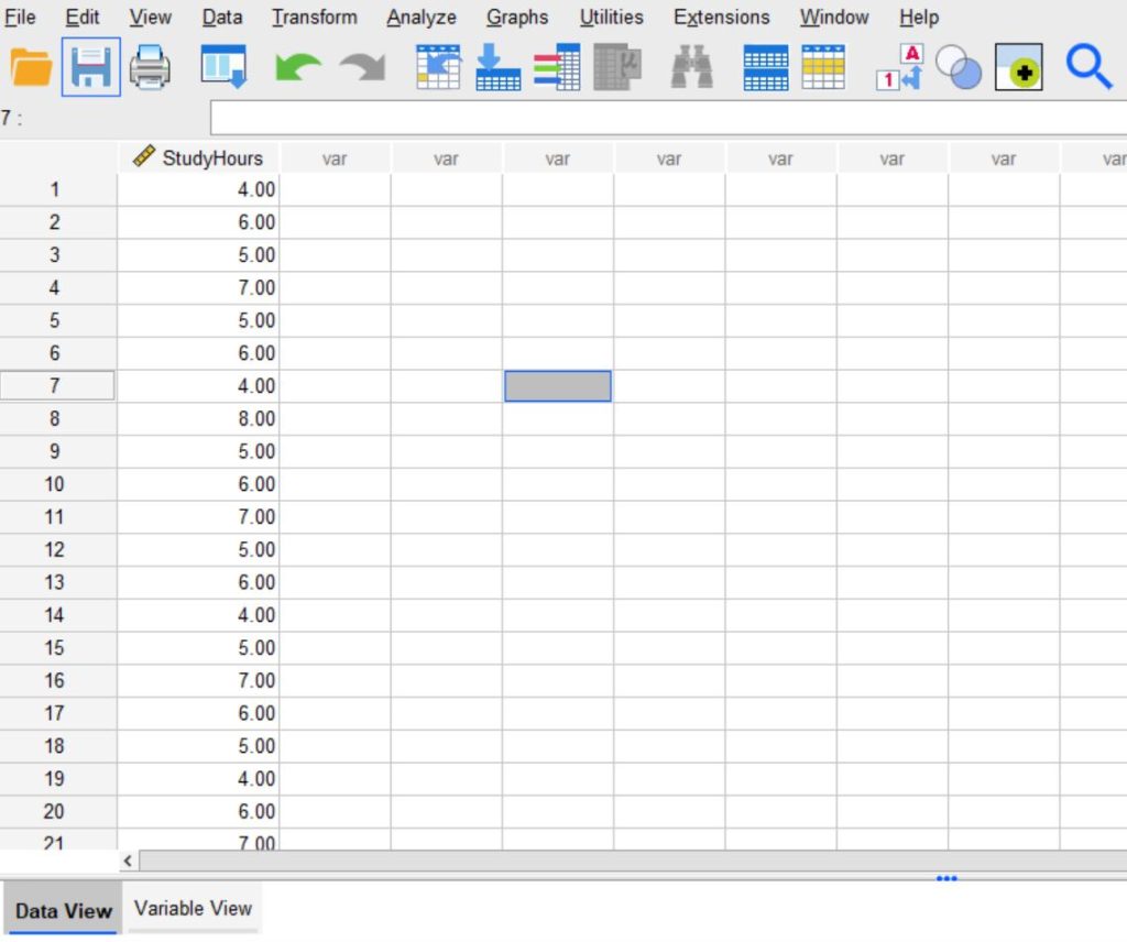
Data View
Next, switch to Data View and enter the study hours for the 30 students. Each row should contain one value for the variable StudyHours.
The Data View should be as shown below.
Alternatively, instead of entering the data manually, you can enter the data in Excel and save it either as CSV or Excel format. You can then use the procedure below to import it into SPSS.
File → Import Data → Excel if you saved it as a .xlsx data, or File → Import Data → CSV Data if you saved it as a .csv data.
Then browse the location and select the Excel or CSV file containing your dataset.
Step 2: Click Analyze → Compare Means → One-Sample T Test
After entering the dataset, go to the top menu bar in SPSS and follow this path:
Analyze → Compare Means → One-Sample T Test
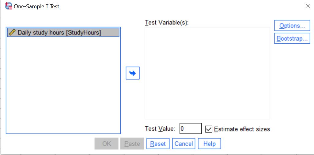
Clicking this option opens the One-Sample T Test dialog box. This window allows you to choose the variable you want to analyze and enter the test value that SPSS will use to compare against the sample mean.
You should see the following dialog box.
Step 3: Select the Test Variable and Enter the Test Value
In the One-Sample T Test dialog box, select the variable you want to analyze and specify the value you want to compare the sample mean against.
First, select the variable StudyHours from the list on the left. Then click the arrow button to move it into the Test Variable(s) box.
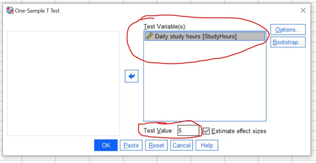
Next, enter the Test Value. The test value is the number that SPSS will use to compare against the sample mean. In this example, the researcher wants to test whether the average study time differs from 5 hours, so the test value is 5.
Therefore, enter:
Test Value = 5
Once you select the test variable and enter the test value, the setup for the one-sample t-test is complete.
The dialog box should be as shown below.
Step 4: Click OK to Run the Test
After selecting the test variable and entering the test value, click OK to run the analysis.
SPSS will process the request and generate the results in the Output Viewer. The output will include tables that summarize the sample statistics and the results of the one-sample t-test.
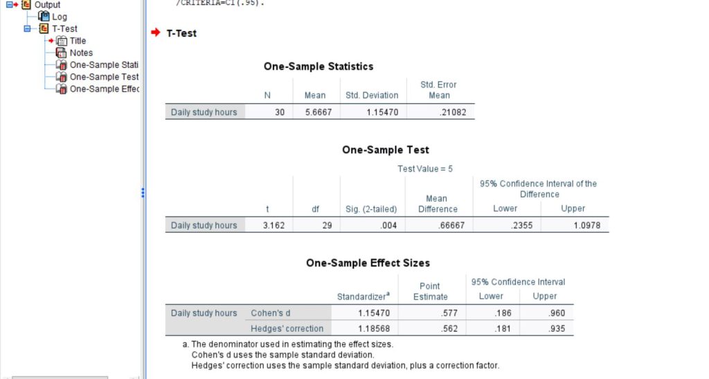
The SPSS output produced for this example is shown below.
Need help running the one-sample t-test in SPSS and writing the results? Get professional SPSS Analysis Help now for high-quality results. Perfect for students and researchers looking for help with running the test, interpreting SPSS outputs, and preparing APA-style reports for assignments, theses, and dissertations.
SPSS Output Tables Explanation
After you run a one-sample t-test in SPSS, the results appear in the Output Viewer. SPSS generates several tables that summarize the data and show the results of the hypothesis test. In this example, the main tables are:
- One-Sample Statistics
- One-Sample Test
- One-Sample Effect Sizes
Each table provides different information that helps you interpret the results.
1. One-Sample Statistics Table
The One-Sample Statistics table summarizes the descriptive statistics of the sample. It shows basic information about the data before the hypothesis test is evaluated.
In this example, the table reports:
- N = 30 → the number of observations included in the analysis
- Mean = 5.6667 → the average study time of the students
- Std. Deviation = 1.15470 → the amount of variation in study hours among the students
- Std. Error Mean = 0.21082 → the estimated standard deviation of the sampling distribution of the mean
This table helps you understand the characteristics of the sample data.
For this study:
- The average study time is about 5.67 hours per day.
- The standard deviation (1.15) shows that study hours vary across students.
- The standard error (0.21) indicates how precisely the sample mean estimates the population mean.
Researchers typically use the mean and standard deviation from this table when reporting results in APA style.
2. One-Sample Test Table
The One-Sample Test table contains the main results of the hypothesis test. It shows whether the sample mean differs significantly from the hypothesized value.
In this example, SPSS compares the sample mean to the test value of 5 hours.
The table includes the following values:
- t = 3.162 → the t-statistic that measures how far the sample mean is from the test value
- df = 29 → the degrees of freedom for the test (calculated as n − 1)
- Sig. (2-tailed) = .004 → the p-value used to determine statistical significance
- Mean Difference = 0.66667 → the difference between the sample mean and the test value
- 95% Confidence Interval = 0.2355 to 1.0978 → the range of plausible values for the true mean difference
These values help determine whether the difference between the sample mean and the hypothesized value is statistically significant.
From the table, we can observe:
- The sample mean is higher than the test value by about 0.67 hours.
- The p-value (.004) is smaller than 0.05, which indicates a statistically significant difference.
- The confidence interval does not include zero, which supports the conclusion that the true mean is different from 5 hours.
This table is the most important table for interpreting the results of the one-sample t-test.
3. One-Sample Effect Sizes Table
The One-Sample Effect Sizes table provides information about the magnitude of the difference between the sample mean and the hypothesized value. While the p-value shows whether the difference is statistically significant, the effect size shows how large the difference is in practical terms.
In this example, SPSS reports two effect size measures:
- Cohen’s d = 0.577
- Hedges’ correction = 0.562
SPSS also provides 95% confidence intervals for these estimates:
- Cohen’s d CI = 0.186 to 0.960
- Hedges’ correction CI = 0.181 to 0.935
These values indicate the strength of the difference between the sample mean and the test value.
Using common interpretation guidelines for Cohen’s d:
- 0.2 → small effect
- 0.5 → medium effect
- 0.8 → large effect
In this example:
- 0.577 indicates a moderate effect size
This means that the difference between the sample mean and the hypothesized value is not only statistically significant but also meaningful in size.
Which Tables Are Most Important?
When interpreting a one-sample t-test in SPSS, focus mainly on these tables:
- One-Sample Statistics → provides the sample mean, standard deviation, and sample size
- One-Sample Test → shows the t-value, degrees of freedom, p-value, mean difference, and confidence interval
- One-Sample Effect Sizes → indicates the practical magnitude of the difference
Together, these tables allow researchers to summarize the sample data, test the hypothesis, and evaluate the practical importance of the results.
How to Interpret One-Sample T-Test Results
To interpret the results of a one-sample t-test, focus on the Sig. (2-tailed) value in the One-Sample T-Test table. This value represents the p-value of the test.
Decision Rule
- If p ≤ 0.05 → there is a statistically significant difference between the sample mean and the test value.
- If p > 0.05 → there is no statistically significant difference.
From the SPSS output:
- Sample mean = 5.67 hours
- Test value = 5 hours
- t(29) = 3.162
- p = 0.004
Since p = 0.004, which is less than 0.05, the result is statistically significant. This means the average study time of the students differs significantly from 5 hours.
Therefore, you can write the interpretation as follows:
The sample mean study time was 5.67 hours per day. A one-sample t-test showed that the average study time of students was significantly higher than 5 hours, t(29) = 3.162, p = 0.004. This result suggests that students in the sample study more than the hypothesized average of 5 hours per day.
Key Takeaways
A one-sample t-test compares the mean of a sample to a known or hypothesized value. Researchers often use this test to determine whether the average of a variable differs significantly from a specific benchmark.
Running a one-sample t-test in SPSS is straightforward. Once your dataset is ready, you only need to follow a few simple steps to perform the analysis and interpret the results.
- Enter the dataset and define the variable in SPSS
- Click Analyze → Compare Means → One-Sample T Test
- Move the variable into the Test Variable(s) box and enter the test value (the hypothesized mean)
- Click OK to run the test
Once you have the outputs, you can either interpret them or write a report in APA style if needed.