How to Run a Chi-Square Test of Independence in SPSS

If you want to know whether two categorical variables are related, a chi-square test of independence is often the right place to start. It is a common test in survey research, health studies, education, business, and social science. The good news is that SPSS makes the procedure fairly straightforward. Once your data is arranged correctly, you can run the test in a few clicks and then focus on understanding the output. That is where many beginners struggle most. This guide shows you exactly how to run a chi-square test of independence in SPSS, how to prepare your data, what options to select, and how to read the results clearly.

If you want the theory behind the test, read our chi-square test of independence guide. However, if you want help writing the findings formally, see our complete tutorial on how to report Chi-Square Results in APA style.

When to Use This Procedure in SPSS

A chi-square test of independence is used when you want to examine whether two categorical variables are associated. In simple terms, it helps you test whether the pattern in one variable differs across categories of another variable.

For example, you may want to know whether gender is related to preferred learning mode, whether smoking status is related to disease status, or whether employment status is related to education level. In each case, the variables are made up of categories rather than numerical scores.

This SPSS procedure is appropriate when:

• You have two categorical variables
• Each participant belongs to one category in each variable
• You want to test whether the two variables are related

This procedure is not appropriate when one of your variables is continuous, when you want to compare means, or when the same person appears in more than one category in a way that breaks independence.

What You Need Before Running the Test

Before opening SPSS, make sure your variables fit the test. This step saves time and helps you avoid confusing output later.

Your two variables should be categorical. That means the values should represent groups or classes, not amounts. Examples include sex, marital status, department, treatment group, and response categories such as yes or no.

You also need independent observations. Each participant should contribute only one response to the cross-tabulation. If the same case is counted more than once in a way that affects the table, the result may be misleading.

Finally, your data should represent frequencies. The chi-square test works with counts of cases in categories. SPSS can handle raw case-level data or already summarized frequency data, but most beginners work with raw data where each row is one participant.

How to Prepare Data for a Chi-Square Test of Independence in SPSS

Many chi-square problems start with data setup rather than with the test itself. If your data is arranged properly, the procedure becomes much easier.

In the most common setup, each row in SPSS represents one case or participant. Each column represents one variable. For a chi-square test of independence, you need one column for the first categorical variable and one column for the second categorical variable.

For example, suppose you want to test whether gender is associated with preferred learning mode. Your data might look like this:

Participant	Gender	Learning_Mode
1	Male	Online
2	Female	Face-to-face
3	Male	Hybrid
4	Female	Online

Each case belongs to one category under Gender and one category under Learning_Mode. That is all SPSS needs to build the crosstab and perform the test.

Coding Categorical Variables Correctly

It is usually best to code categories with numbers in SPSS and then assign value labels. This keeps your data clean and makes the output easier to read.

For example, you might code Gender like this:

• 1 = Male
• 2 = Female

You might code Learning Mode like this:

• 1 = Online
• 2 = Face-to-face
• 3 = Hybrid

The numeric codes themselves do not affect the chi-square result. They simply help SPSS store the categories. What matters is that each code represents a distinct category and that the labels are entered correctly in Variable View.

Avoid using continuous variables as if they were categorical unless you have a clear reason for grouping them. Also, avoid inconsistent coding, such as using 1 and 2 for one case and text labels for another. Clean coding leads to cleaner output.

If You Have Frequency Data Instead of Raw Cases

Sometimes you may not have one row per participant. Instead, you may already have a summary table showing counts for category combinations. SPSS can still run the analysis, but you need to weight the data first.

In this situation, your dataset usually has one column for the first variable, one column for the second variable, and one column for the frequency count. You would then tell SPSS to weight cases by that frequency variable before running the crosstabs procedure.

Many students do not need this step because their datasets already contain raw responses. Still, it is helpful to know that SPSS can handle both formats.

If you are unsure, check your file. If each row is one participant, you likely do not need weighting. However, if each row is one combination of categories with a count attached, then weighting may be necessary before running the chi-square test.

Assumptions to Check Before Running the Test

The chi-square test of independence is not difficult, but it does have important assumptions. You do not need to turn this into a highly technical exercise, but you should know what to check before trusting the result.

The first assumption is independence of observations. Each case should contribute to only one cell in the table. For example, if one student answers the survey once, that is fine. If the same student is counted multiple times in a way that affects the crosstab, the assumption is violated.

The second assumption concerns expected cell counts. The test works best when the expected frequencies are not too small. SPSS helps you check this in the output, so you do not need to calculate everything by hand.

When assumptions are badly violated, the p-value may not be reliable. That is why you should always look beyond the main significance value and check the footnotes and supporting tables as well.

Understanding Expected Cell Counts

Expected counts are the frequencies SPSS would expect in each cell if the two variables were unrelated. The chi-square test compares these expected counts with the observed counts in your table.

In practice, you do not need to compute them manually because SPSS provides them in the crosstab output when you request them. What matters is knowing whether the expected frequencies are large enough for the test to be trustworthy.

A common guideline is that no expected count should be below 1, and no more than 20% of the cells should have expected counts below 5 in larger tables. In small 2×2 tables, very low expected counts are a stronger concern.

Do not panic if you see a warning. It does not always mean the analysis is useless. It simply means you need to interpret carefully and possibly consider an alternative, such as Fisher’s exact test for small 2×2 tables.

How to Run a Chi-Square Test of Independence in SPSS

Once your data is ready, the procedure in SPSS is simple. The key is knowing which options to select so that the output gives you what you need for interpretation.

In SPSS, the chi-square test of independence is usually run through the Crosstabs dialog box. That is where you place your variables, request the chi-square statistic, and choose the cell information that helps you understand the relationship.

The test itself is quick. Most of the value comes from setting up the output properly. That is why you should ask SPSS to show observed counts, expected counts, and row or column percentages. These details help you explain what the association actually looks like instead of reporting only that it is significant or not significant.

Follow the steps below carefully.

Step 1: Open the Crosstabs Dialog Box

Start from the top menu in SPSS:

Analyze > Descriptive Statistics > Crosstabs

This opens the Crosstabs window. It is the main area used to run a chi-square test of independence in SPSS.

You will see boxes labeled Row(s) and Column(s). This is where you place the two categorical variables you want to test. You will also see buttons for Statistics, Cells, and Format.

At this stage, do not worry too much about which variable goes in rows and which goes in columns. The chi-square significance result will be the same either way. However, the arrangement can affect how easy it is to interpret percentages. Try to place the variable you want to compare across categories in the position that makes the output more readable.

Step 2: Move Your Variables into Rows and Columns

Select one categorical variable and move it into the Row(s) box. Select the other categorical variable and move it into the Column(s) box.

For example, if you are testing whether gender is related to preferred learning mode, you might place Gender in Rows and Learning_Mode in Columns. SPSS will then produce a table showing how the learning mode categories are distributed across gender categories.

The test result will not change if you swap them, but the percentages may be easier to understand one way rather than the other. In many cases, researchers prefer to place the explanatory or grouping variable in rows and the outcome-like category variable in columns, but there is no strict rule.

The important thing is to be consistent and to arrange the table in a way that helps readers follow the pattern.

Step 3: Request the Chi-Square Statistic

After placing your variables in the Crosstabs dialog box, click the Statistics button.

A smaller window will open with a list of options. Tick Chi-square. This tells SPSS to compute the chi-square test of independence.

You should also tick Phi and Cramer’s V. These measures help you understand the strength of the relationship. They are especially useful because the p-value alone only tells you whether there is evidence of an association, not how strong that association is.

After selecting these options, click Continue to return to the main Crosstabs window.

This is a small but important step. Beginners often request only the chi-square test and then realize later that they also need an effect size measure.

Step 4: Choose the Right Cell Options

Next, click the Cells button. This is where you control what information appears inside the crosstab table.

Under counts, tick:

• Observed
• Expected

Under percentages, tick either:

• Row percentages
• or Column percentages

You can choose both, but for beginners that can make the table look crowded. It is often better to choose the one that best matches your research question.

If you want to compare the distribution across row groups, row percentages are usually easier to interpret. If you want to compare within columns, column percentages may be better.

Click Continue after making your selections. These options will make your output much more informative.

Step 5: Run the Analysis

Once everything is set, click OK in the main Crosstabs window.

SPSS will generate the output in the Output Viewer. You will usually see several tables, including:

• Case Processing Summary
• Crosstabulation
• Chi-Square Tests
• Symmetric Measures

Do not rush straight to the p-value. A good interpretation starts with checking the number of valid cases, then studying the crosstab, and finally examining the test results and assumptions.

That order helps you avoid mistakes and gives you a much clearer understanding of what your data is showing.

How to Read the Output in SPSS

Many users can click through the SPSS menus, but they get stuck when the output appears. That is normal. The good news is that once you know what each table is doing, the results become much easier to follow.

A chi-square output is not just one number. You need to read the output in pieces. Start with the number of valid cases. Then look at the crosstab to understand the pattern in the data. After that, move to the chi-square test table to check whether the association is statistically significant. Finally, look at the effect size and expected count notes.

This sequence helps you move from the basic data structure to the statistical conclusion in a sensible way.

Case Processing Summary

The Case Processing Summary tells you how many cases were included in the analysis and how many were missing.

This is a quick but useful table. It helps you confirm that SPSS used the number of cases you expected. If the valid count is much lower than your sample size, you may have missing data in one or both variables.

Always check this table before interpreting the rest of the output. A large amount of missing data can affect how representative your findings are.

If the number of valid cases looks correct, you can move on with more confidence. If it does not, go back and inspect your dataset for missing values, miscoding, or data entry problems.

Crosstabulation Table

The Crosstabulation table is one of the most important parts of the output because it shows the actual pattern of the relationship.

Here you will see the observed counts for each combination of categories. If you requested expected counts, those will also appear. If you selected row or column percentages, SPSS will display them as well.

This table helps you answer questions such as:

• Which group has the highest proportion in a category?
• Where do the observed counts differ most from the expected counts?
• Is the pattern strong or only slight?

Even when the chi-square test is significant, you still need this table to explain what the relationship looks like. The p-value tells you that an association exists. The crosstab shows where that association appears in the data.

Chi-Square Tests Table

The Chi-Square Tests table contains the main statistical test result. In most basic interpretations, the key line to focus on is Pearson Chi-Square.

This row provides the chi-square statistic, the degrees of freedom, and the p-value. The p-value tells you whether the association between the two categorical variables is statistically significant.

If the p-value is less than your chosen significance level, usually .05, you conclude that there is a statistically significant association between the variables. If it is greater than .05, you conclude that there is not enough evidence to say the variables are associated.

Do not stop at significance alone. A significant result does not tell you how strong the relationship is, and it does not tell you which categories are driving the pattern. That is why the crosstab and effect size table are also important.

Symmetric Measures Table

The Symmetric Measures table provides effect size statistics that help describe the strength of the association.

If your table is 2×2, you will often look at Phi. If your table is larger than 2×2, Cramer’s V is usually the more appropriate measure.

These statistics range from 0 upward, with larger values indicating a stronger association. The exact interpretation depends on the context and the table size, so avoid treating them too mechanically. Still, they are useful for showing that statistical significance and practical strength are not the same thing.

A large sample can produce a significant p-value even when the relationship is weak. That is why effect size matters. It helps you describe the importance of the result more clearly.

Expected Count Footnote

At the bottom of the chi-square output, SPSS often includes a footnote about expected counts. Do not ignore it.

This note tells you whether any cells had expected counts that were too small for the chi-square approximation to be fully reliable. You may see wording such as the number or percentage of cells with expected counts below 5, along with the minimum expected count.

If the warning is mild and the assumptions are still reasonably met, you may proceed with caution. If many expected counts are too small, the chi-square result may not be the best choice for that table.

This is one reason you should not rely only on the Pearson chi-square p-value. Good interpretation includes checking whether the test assumptions were satisfied.

A Worked Example

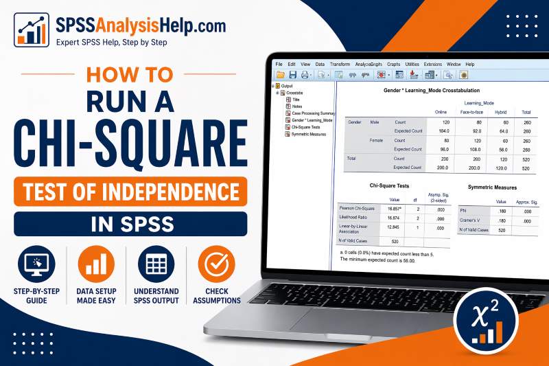
Suppose a researcher wants to know whether gender is associated with preferred learning mode among university students. Gender has two categories: male and female. Preferred learning mode has three categories: online, face-to-face, and hybrid.

The researcher enters the data into SPSS so that each row represents one student. Gender is placed in one column and learning mode in another. Then the researcher opens Analyze > Descriptive Statistics > Crosstabs, places Gender in Rows and Learning Mode in Columns, selects Chi-square under Statistics, and chooses Observed, Expected, and Row percentages under Cells.

After running the test, SPSS produces the crosstab and chi-square tables. The researcher first checks the Case Processing Summary, then studies the row percentages in the crosstab to see how learning mode preferences differ by gender. Next, the researcher looks at the Pearson chi-square p-value to determine whether the association is statistically significant. Finally, the researcher checks Cramer’s V to understand the strength of the relationship and reviews the expected count footnote to confirm that the test assumptions were acceptable.

How to Interpret the Example in Plain Language

Imagine the crosstab shows that a higher percentage of male students prefer online learning, while a higher percentage of female students prefer face-to-face learning. The hybrid option is distributed more evenly.

If the Pearson chi-square p-value is below .05, the researcher concludes that the preferred learning mode is significantly associated with gender. In plain language, this means the distribution of learning preferences differs by gender more than would be expected by chance alone.

The crosstab tells the story of how the categories differ. The chi-square p-value tells you whether the difference is statistically significant. The effect size tells you whether the relationship is weak or stronger in practical terms.

This is the kind of interpretation beginners should aim for. Keep it simple, accurate, and tied to what the tables actually show.

What to Do If Expected Counts Are Too Small

Sometimes SPSS will warn that the expected counts are too low. This often happens when your sample size is small or when you have too many categories with very few cases in some cells.

If you are working with a 2×2 table, one possible alternative is Fisher’s exact test. This test is often more appropriate when expected frequencies are very small. It is especially useful in small samples.

Another option is to combine sparse categories, but only when that decision makes substantive sense. Do not merge categories just to make the numbers look better. The revised categories should still reflect a meaningful variable structure.

The key point is simple: do not ignore the warning. A chi-square result is only as trustworthy as the assumptions behind it.

Common Mistakes When Running Chi-Square in SPSS

Beginners often make similar mistakes with chi-square tests. Once you know them, they are much easier to avoid.

One common mistake is using the wrong type of variable. If one of your variables is continuous, the chi-square test of independence is usually not appropriate unless the variable has been carefully categorized.

Another mistake is forgetting to request expected counts. Without them, it becomes harder to check whether the assumptions are met.

Some users also focus only on the p-value and ignore the crosstab. That leads to a weak interpretation because the significance test alone does not show the pattern in the data.

A further mistake is confusing the chi-square test of independence with the chi-square goodness-of-fit test. They are related but used for different purposes.

SPSS Syntax for a Chi-Square Test of Independence

Some users prefer syntax because it makes analysis more reproducible. It also helps if you need to rerun the same procedure later.

Here is a simple example of SPSS syntax for a chi-square test of independence:

CROSSTABS
  /TABLES=Gender BY Learning_Mode
  /FORMAT=AVALUE TABLES
  /STATISTICS=CHISQ PHI
  /CELLS=COUNT EXPECTED ROW
  /COUNT ROUND CELL.

In this example, SPSS produces a crosstab of Gender by Learning_Mode, computes the chi-square test, and displays observed counts, expected counts, and row percentages.

Syntax is not required for beginners, but it is useful if you want a clear record of the steps you used.

Final Thoughts

Running a chi-square test of independence in SPSS is not difficult once your data is arranged correctly and you know which options to select. The main steps are simple: prepare the data, open Crosstabs, request the chi-square statistic, display expected counts and percentages, and then read the output carefully.

The most important habit is to go beyond the p-value. Always inspect the crosstab, check the expected count note, and look at the effect size. That gives you a fuller and more accurate interpretation.

Frequently Asked Questions