How to Run a Chi-Square Goodness of Fit Test in SPSS

Running a chi-square goodness-of-fit test in SPSS is useful when you want to compare observed category counts with expected category counts. For example, you may want to test whether students prefer online, hybrid, and face-to-face classes equally. You may also want to test whether responses in a survey match expected percentages.

This guide focuses on the practical SPSS steps. You will learn how to prepare your data, when to weight cases, how to enter expected values, how to run the test, and how to read the SPSS output.

However, if you are comparing two categorical variables, this is not the right test. In that case, read our guide on how to run a chi-square test of independence in SPSS.

When This SPSS Procedure Is Appropriate

Use the chi-square goodness of fit procedure in SPSS when your analysis has one categorical variable.

Your data should contain categories such as:

• learning mode;
• product choice;
• response option;
• department;
• preference group;
• customer type;
• political choice;
• diagnosis group.

The test compares the number of cases observed in each category with the number expected in each category. For example, suppose 120 students choose one preferred study mode. The categories are online, hybrid, and face-to-face. If you expect equal preference, SPSS compares the observed counts with 40, 40, and 40.

---

Before You Start: Check Your Data Format

Before opening the chi-square test dialog box, you need to know how your data are arranged.

SPSS data for this test usually come in one of two formats:

Data Format	What Each Row Represents	Do You Weight Cases?
Raw data	One participant or case	No
Frequency data	One category and its count	Yes

This step matters because SPSS treats each row as one case unless you tell it otherwise.

If your file has 120 rows for 120 students, that is raw data. You should not weight cases. However, if your file has only three rows, such as Online = 50, Hybrid = 42, Face-to-face = 28, that is frequency data. You must weight cases before running the test.

Many wrong chi-square results in SPSS come from skipping this step.

Example Used in This SPSS Tutorial

We will use the same example throughout the guide.

A university surveys 120 students about their preferred study mode. The results are shown below.

Study Mode	Observed Frequency
Online	50
Hybrid	42
Face-to-face	28
Total	120

The question is:

Are students equally likely to prefer online, hybrid, and face-to-face learning?

If the three categories are expected to be equal, each category should have:

120 ÷ 3 = 40

So, the expected frequencies are:

Study Mode	Expected Frequency
Online	40
Hybrid	40
Face-to-face	40

We will use this example to show the data setup, SPSS steps, and output interpretation.

---

How to Enter Raw Data in SPSS

Raw data means each row represents one participant or case.

Your SPSS Data View may look like this:

ID	Study_Mode
1	Online
2	Hybrid
3	Online
4	Face-to-face
5	Hybrid

In this setup, each student appears in a separate row. The variable Study_Mode records the category selected by each student.

If your data are in this format, SPSS can count the categories automatically. You do not need to weight cases.

It is still a good idea to use numeric codes and value labels. For example:

Code	Label
1	Online
2	Hybrid
3	Face-to-face

This makes your output easier to read.

If your categories need to be cleaned or recoded first, see our guide on how to recode variables in SPSS.

---

How to Enter Frequency Data in SPSS

Frequency data means your data are already summarized as counts.

Your SPSS Data View may look like this:

Study_Mode	Count
Online	50
Hybrid	42
Face-to-face	28

In this format, each row is not one student. Each row is one category.

This means SPSS will not automatically know that Online represents 50 students unless you weight cases.

If you run the test without weighting cases, SPSS may treat the file as if it has only three cases. That will give an incorrect result.

For frequency data, you need two variables:

Variable	Purpose
Study_Mode	Shows the category
Count	Shows the number of cases in that category

After entering the data, you must weight cases by the count variable before running the chi-square goodness of fit test.

---

How to Weight Cases in SPSS

Use this step only if your data are summarized as frequencies.

To weight cases in SPSS:

1. Click Data.
2. Select Weight Cases.
3. Choose Weight cases by.
4. Move your frequency variable, such as Count, into the Frequency Variable box.
5. Click OK.

SPSS will now treat each category as having the correct number of cases.

For example:

Study Mode	Count
Online	50
Hybrid	42
Face-to-face	28

After weighting, SPSS reads this as 50 online cases, 42 hybrid cases, and 28 face-to-face cases.

After completing your analysis, turn weighting off if you plan to run other tests.

To turn weighting off:

1. Click Data.
2. Select Weight Cases.
3. Choose Do not weight cases.
4. Click OK.

This prevents mistakes in later analyses.

---

How to Run the Chi-Square Goodness of Fit Test in SPSS

After your data are ready, follow these steps:

1. Click Analyze.
2. Select Nonparametric Tests.
3. Select Legacy Dialogs.
4. Click Chi-Square.

The Chi-Square Test dialog box will appear.

Next:

1. Move your categorical variable into the Test Variable List box.
2. Go to the Expected Values section.
3. Choose All categories equal or Values.
4. Click OK.

For our example, the categorical variable is Study_Mode.

Because we want to test whether students are equally likely to choose the three study modes, we choose All categories equal.

SPSS will then compare the observed frequencies with equal expected frequencies.

---

Choosing the Correct Expected Values

The expected values tell SPSS what pattern you want to compare your observed data against.

SPSS gives you two choices:

Option	When to Use It
All categories equal	When each category is expected to have the same frequency
Values	When categories have different expected frequencies

Choosing the correct option is important. The output depends on the expected values you enter.

For example, testing whether three categories are equally common is different from testing whether the categories follow a 50%, 30%, and 20% pattern.

Before you click OK, ask yourself:

What should the distribution look like if the null hypothesis is true?

If the categories should be equal, choose All categories equal.

If the categories should follow specific proportions or counts, choose Values.

---

Option 1: All Categories Equal

Choose All categories equal when every category should have the same expected frequency.

In our example, there are 120 students and 3 study modes:

Study Mode	Expected Frequency
Online	40
Hybrid	40
Face-to-face	40

You do not need to enter 40, 40, and 40 manually. SPSS calculates equal expected frequencies automatically.

Use this option when your research question is like:

• Are customers equally likely to choose each product?
• Are students equally likely to select each learning mode?
• Are responses evenly distributed across categories?
• Are participants equally likely to choose each option?

This is the most common option in many beginner SPSS assignments.

---

Option 2: Unequal Expected Values

Choose Values when your categories are expected to occur in different proportions.

For example, suppose previous data suggest that student preferences should follow this pattern:

Study Mode	Expected Proportion
Online	50%
Hybrid	30%
Face-to-face	20%

For a sample of 120 students, the expected counts would be:

Study Mode	Expected Count
Online	60
Hybrid	36
Face-to-face	24

In SPSS, choose Values and enter:

60, 36, 24

Click Add after each value if SPSS requires it.

Make sure the values are entered in the same order as the categories in your dataset. If the order is wrong, SPSS will match the expected counts to the wrong groups.

---

Check the Category Order Before Entering Expected Values

This step is very important when using unequal expected values.

SPSS matches the expected values to categories based on the category order.

Suppose your categories are coded like this:

Code	Label
1	Online
2	Hybrid
3	Face-to-face

If the expected counts are Online = 60, Hybrid = 36, and Face-to-face = 24, enter:

60, 36, 24

However, suppose your coding is different:

Code	Label
1	Face-to-face
2	Hybrid
3	Online

Now the correct order would be:

24, 36, 60

This is a common SPSS mistake. Always check your coding in Variable View before entering unequal expected values.

---

SPSS Output: What Tables to Look At

After running the test, SPSS will usually produce two important output tables:

1. Frequencies
2. Test Statistics

The Frequencies table helps you compare the observed and expected counts.

The Test Statistics table gives the chi-square value, degrees of freedom, and p-value.

You should not look at the p-value only. First, check the Frequencies table to see whether SPSS used the correct observed and expected counts.

This is especially important if you weighted cases or entered unequal expected values.

If the observed counts look wrong, go back and check your data setup. If the expected counts look wrong, check your expected values and category order.

Once the counts look correct, you can interpret the test result.

---

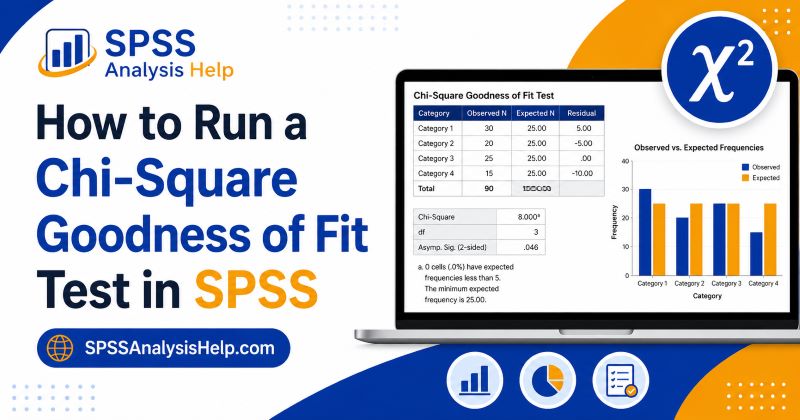
How to Read the Frequencies Table

The Frequencies table usually contains these columns:

Column	Meaning
Observed N	The actual count in each category
Expected N	The expected count in each category
Residual	Observed N minus Expected N

Using our example, the table may look like this:

Study Mode	Observed N	Expected N	Residual
Online	50	40	10
Hybrid	42	40	2
Face-to-face	28	40	-12

The residual shows how far each observed count is from its expected count.

A positive residual means the category had more cases than expected.

A negative residual means the category had fewer cases than expected.

In this example, Online had 10 more students than expected. Face-to-face had 12 fewer students than expected.

---

How to Read the Test Statistics Table

The Test Statistics table gives the main result of the analysis.

You will usually see:

SPSS Output Term	Meaning
Chi-Square	The test statistic
df	Degrees of freedom
Asymp. Sig.	The p-value

The Chi-Square value shows the overall difference between observed and expected frequencies.

The df value means degrees of freedom. For a goodness of fit test, this is usually:

df = number of categories − 1

In our example:

df = 3 − 1 = 2

The Asymp. Sig. value is the p-value.

Use this rule:

• If p < .05, the result is statistically significant.
• If p ≥ .05, the result is not statistically significant.

If your instructor gives a different alpha level, use that instead.

---

How to Interpret a Significant Result in SPSS

A significant result means the observed frequencies are different from the expected frequencies.

For example, if SPSS gives a p-value below .05, you reject the null hypothesis.

In simple language, you could say:

The distribution of student study mode preferences was significantly different from the expected equal distribution.

Then look at the residuals to describe the pattern.

Using our example:

• Online had more students than expected.
• Hybrid was close to the expected count.
• Face-to-face had fewer students than expected.

This helps you explain where the difference appears.

However, be careful. The chi-square goodness of fit test tells you that the overall distribution differs from expectation. It does not explain why the difference happened.

---

How to Interpret a Non-Significant Result in SPSS

A non-significant result means the observed frequencies are not different enough from the expected frequencies to be considered statistically significant.

For example, if SPSS gives a p-value of .05 or higher, you fail to reject the null hypothesis.

In simple language, you could say:

There was not enough evidence to conclude that student study mode preferences differed from the expected equal distribution.

This does not mean the observed counts are exactly equal. It only means the difference was not statistically significant.

For example, you may still see small differences between observed and expected counts. However, those differences may be small enough to occur by chance.

Always avoid saying that the null hypothesis is “proven true.” It is better to say that the result was not statistically significant.

---

Worked SPSS Example

Let us walk through the full process using our example.

A university surveyed 120 students about preferred study mode.

Study Mode	Observed Frequency
Online	50
Hybrid	42
Face-to-face	28

The university wants to test whether the three study modes are selected equally.

Because the data are summarized, enter them into SPSS like this:

Study_Mode	Count
Online	50
Hybrid	42
Face-to-face	28

Then weight cases by Count.

Next, go to:

Analyze > Nonparametric Tests > Legacy Dialogs > Chi-Square

Move Study_Mode into the Test Variable List box.

Under Expected Values, choose All categories equal.

Click OK.

In the output, check the Frequencies table first. Confirm that the observed counts are 50, 42, and 28. Then check that the expected counts are 40, 40, and 40.

Finally, read the p-value in the Test Statistics table.

---

SPSS Syntax for Chi-Square Goodness of Fit Test

You can also run the test using SPSS syntax.

For equal expected frequencies, use:

NPAR TESTS
  /CHISQUARE = Study_Mode
  /EXPECTED = EQUAL.

This compares the observed category counts with equal expected counts.

For unequal expected frequencies, use:

NPAR TESTS
  /CHISQUARE = Study_Mode
  /EXPECTED = 60 36 24.

This compares the observed counts with expected counts of 60, 36, and 24.

Make sure the expected values are in the correct category order.

If you weighted frequency data, your syntax may also include a weight command such as:

WEIGHT BY Count.

After finishing, you can turn weights off using:

WEIGHT OFF.

Syntax is useful because it keeps a clear record of the analysis.

---

Common SPSS Mistakes to Avoid

Here are common mistakes students make when running a chi-square goodness-of-fit test in SPSS.

• Forgetting to Weight Frequency Data. If your file contains summarized counts, you must weight cases. Otherwise, SPSS may treat each row as one case.
• Weighting Raw Data. If each row is already one participant, do not weight cases.
• Choosing the Wrong Expected Values. Use All categories equal only when the expected distribution is equal. Use Values when the expected distribution is unequal.
• Entering Expected Values in the Wrong Order. When using unequal expected values, always check the category coding first.
• Using the Wrong Chi-Square Procedure. If you have two categorical variables, use the chi-square test of independence instead.
• Ignoring the Frequencies Table. Always check whether SPSS used the correct observed and expected counts before interpreting the p-value.

---

What to Do If the Output Looks Wrong

Sometimes the SPSS output does not match what you expected. This often happens because of data setup problems.

Check the following:

• Did you weight cases when using frequency data?
• Did you forget to turn weighting off from a previous analysis?
• Did you move the correct variable into the Test Variable List?
• Did you enter expected values in the correct order?
• Did you use raw counts instead of percentages?
• Did your category labels match your coding?

If the observed counts are wrong, check your data entry or weighting. If the expected counts are wrong, check your expected values. However, if the p-value seems unusual, do not change the result. Go back and confirm that the data and settings are correct.

---

Brief Note on Reporting the Result

This article focuses on running the test in SPSS and interpreting the output. After you get your result, you may need to write it in APA style. The APA write-up usually includes the chi-square value, degrees of freedom, sample size, p-value, and a short interpretation.

Since that is a separate topic, we have covered it in another article. You can read our guide on how to report chi-square test results in APA style.

That guide is more useful once you already have your SPSS output and want to present the result correctly in an assignment, dissertation, thesis, or research report.

---

Final Thoughts

To run a chi-square goodness-of-fit test in SPSS, start by checking your data format. If each row is one participant, use the data as it is. If your data are summarized as counts, weight cases first.

Then open the chi-square test through:

Analyze > Nonparametric Tests > Legacy Dialogs > Chi-Square

Move your categorical variable into the Test Variable List, choose the correct expected values, and run the test.

After SPSS produces the output, check the Frequencies table first. Make sure the observed and expected counts are correct. Then use the Test Statistics table to interpret the chi-square value, degrees of freedom, and p-value.

The most important point is this: correct data setup comes before correct interpretation.

Need Help Running a Chi-Square Goodness of Fit Test in SPSS?

The chi-square goodness of fit test is easy to run once your data are set up correctly. However, mistakes in weighting cases, expected values, or category coding can lead to wrong results.

At SPSSAnalysisHelp, we help students and researchers run SPSS analyses, interpret output, and explain results clearly.

You may need help if:

• You are not sure whether to weight cases.
• Your expected values are unequal.
• Your SPSS output looks confusing.
• You do not know which chi-square test to use.
• You need help explaining the result in your assignment or dissertation.

You can explore our SPSS data analysis help, SPSS help for students, data analysis assignment help, or dissertation statistics help services.

---

Frequently Asked Questions