Chi-Square Test of Independence: Definition, Formula, Assumptions, and Examples

Understanding relationships in categorical data is an important part of statistics. In many research projects, the goal is not to compare means. Instead, the goal is to find out whether two categories are related. That is where the chi-square test of independence becomes useful. This test helps you examine whether there is a statistically significant association between two categorical variables. For example, you may want to know whether gender is related to voting preference, whether education level is related to employment status, or whether treatment group is related to recovery category. The chi-square test of independence is designed for exactly that purpose.

In this guide, you will learn what the chi-square test of independence is, when to use it, how it works, what assumptions it requires, and how to interpret the results. You will also see a simple example that makes the ideas easier to follow.

If you want the practical software steps, read our guide on how to run a chi-square test of independence in SPSS. If you want help presenting your findings, see our guide on how to report chi-square results in APA style.

What is a Chi-Square Test of Independence?

The chi-square test of independence is a nonparametric statistical test used to determine whether two categorical variables are associated. In simple terms, it checks whether the pattern of one variable depends on the pattern of another variable.

Suppose you survey students and record their gender and preferred mode of learning. If the preference for online, hybrid, or face-to-face learning differs across gender groups, the two variables may be associated. If the pattern is similar across groups, the variables may be independent.

The word independence is very important here. If two variables are independent, knowing the value of one variable does not help you predict the value of the other. If they are not independent, then some relationship exists between them.

This test is also called the chi-square test of association or the Pearson chi-square test of independence. These names often refer to the same idea in introductory statistics.

Why This Test Matters

Many real-world research questions involve categories rather than numerical scores. A researcher may want to know whether smoking status is associated with disease status, whether marital status is related to job satisfaction category, or whether department is linked to employee turnover intention category.

The chi-square test of independence gives you a way to test these questions formally. Instead of relying on guesswork or visual inspection alone, you can use a statistical test to decide whether the association in your sample is likely to reflect a real pattern in the population.

This makes the test valuable in education, public health, psychology, sociology, business, and many other fields. It is especially useful when data are organized into counts within a contingency table.

When to Use the Chi-Square Test of Independence

You should use the chi-square test of independence when you have two categorical variables and want to know whether they are related. Both variables should consist of categories, not continuous measurements.

Examples include:

• gender and product preference
• religion and voting choice
• education level and employment status
• treatment group and outcome category

The data should be presented as frequencies or counts. That means each cell in the table shows how many cases fall into that combination of categories.

The test is commonly used when your data are summarized in a contingency table, also called a crosstab. This table shows the count of observations for each combination of row and column categories.

If your variables are continuous, or if your goal is to compare averages, then this is not the correct test.

Situations Where This Test Is Appropriate

The chi-square test of independence is appropriate when:

• Both variables are categorical
• The observations come from one sample
• Each case belongs to only one category for each variable
• The data are frequency counts
• You want to test whether the variables are associated

A common student mistake is to choose this test simply because the data can be placed in rows and columns. That is not enough. The variables must truly be categorical, and the numbers in the table must represent counts of cases.

Situations Where This Test Is Not Appropriate

This test is not appropriate when:

• One or both variables are continuous
• The observations are paired or repeated
• The table contains percentages instead of counts
• The expected frequencies are too small in too many cells
• The data come from matched subjects rather than independent observations

In small-sample situations, especially for a 2×2 table, Fisher’s exact test may be more appropriate than the chi-square test.

What Does Independence Mean?

In statistics, independence means that the distribution of one variable does not change across the categories of another variable. If two variables are independent, then they do not show a systematic relationship.

For example, imagine a study that records eye color and preference for tea or coffee. If the proportion of tea and coffee drinkers is about the same across all eye color groups, then the variables appear independent. Eye color would not seem related to beverage preference.

Now, imagine a different study where job role and remote work preference are examined. If managers strongly prefer hybrid work while support staff mainly prefer fully remote work, there may be an association. In that case, the variables are not independent.

The chi-square test of independence helps you test this idea using sample data.

The Hypotheses for a Chi-Square Test of Independence

Like many statistical tests, the chi-square test of independence begins with a null hypothesis and an alternative hypothesis.

Null Hypothesis

The null hypothesis states that the two categorical variables are independent. In other words, there is no association between them in the population.

You can write it like this:

H0: There is no association between the two categorical variables.

Alternative Hypothesis

The alternative hypothesis states that the two variables are not independent. This means there is an association between them in the population.

You can write it like this:

H1: There is an association between the two categorical variables.

The test does not tell you why the association exists. It only tells you whether the observed pattern is strong enough to suggest that a relationship is present.

Understanding the Contingency Table

The chi-square test of independence is based on a contingency table. This table organizes data into rows and columns so you can see how often each combination of categories occurs.

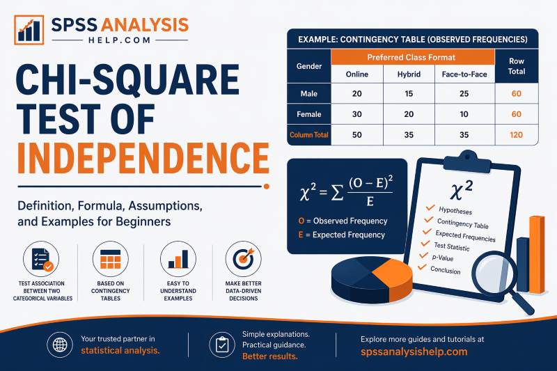
Suppose you survey 120 students about gender and preferred class format. A contingency table can show how many male and female students prefer online, hybrid, or face-to-face learning.

Gender	Online	Hybrid	Face-to-Face	Row Total
Male	20	15	25	60
Female	30	20	10	60
Column Total	50	35	35	120

Each number inside the table is called a cell frequency. These are the actual observed counts from your sample. For example, 25 in the male face-to-face cell means that 25 male students preferred face-to-face classes.

The rows usually represent one categorical variable, and the columns represent the other. Row totals, column totals, and the grand total are also important because they are used to calculate expected frequencies.

Observed Frequencies

Observed frequencies are the actual counts you collected. These are the values that appear in the cells of your contingency table.

For example, if 25 male students prefer online learning, then 25 is an observed frequency.

Expected Frequencies

Expected frequencies are the counts you would expect in each cell if the two variables were completely independent.

These expected values are not guessed. They are calculated from the row totals, column totals, and grand total. The chi-square test compares the observed frequencies to the expected frequencies. If the differences are large, the test statistic becomes larger, and evidence against the null hypothesis increases.

The Chi-Square Test of Independence Formula

The chi-square statistic is calculated using this formula:

χ² = Σ (O − E)² / E

Where:

• O = observed frequency
• E = expected frequency
• Σ = sum across all cells in the table

The formula measures how far the observed counts are from the expected counts. If observed and expected values are very close, the chi-square value will be small. If they differ a lot, the chi-square value will be large.

A large chi-square statistic suggests that the observed pattern is unlikely to have happened by chance alone if the variables were truly independent.

Formula for Expected Frequency

The expected frequency for each cell is calculated as:

Expected frequency = (Row total × Column total) / Grand total

This formula tells you what count you would expect in that cell if the row and column variables had no relationship.

Degrees of Freedom

The degrees of freedom for a chi-square test of independence are calculated as:

df = (r − 1)(c − 1)

Where:

• r = number of rows
• c = number of columns

Degrees of freedom are needed to determine the p-value for the test.

Assumptions of the Chi-Square Test of Independence

Before using this test, you should make sure its assumptions are met. Ignoring assumptions can lead to misleading conclusions.

The Variables Must Be Categorical

Both variables must be categorical. This means the values should fall into groups such as male/female, yes/no, employed/unemployed, or high/medium/low.

If your data are numerical measurements like age, income, or test score, this test is not appropriate unless those values have been meaningfully grouped into categories.

Observations Must Be Independent

Each observation should belong to only one cell in the table. One participant should not be counted more than once in a way that creates dependence between observations.

For example, if the same person answers the survey twice, or if matched pairs are used, the independence assumption is violated.

Data Must Be Frequency Counts

The values in the table should be counts of cases, not percentages, means, or scores. A chi-square test works with raw frequencies.

You may report percentages later to help interpretation, but the actual test should be based on counts.

Expected Cell Counts Must Be Adequate

Expected frequencies should not be too small. A common guideline is that no expected cell count should be less than 1, and no more than 20% of the cells should have expected counts below 5.

If this assumption is badly violated, the chi-square approximation may not be reliable. In such cases, combining categories or using Fisher’s exact test may be better.

How the Chi-Square Test of Independence Works

Once your data are in a contingency table, the logic of the test is straightforward. The test asks one main question: are the observed counts different enough from the expected counts to suggest a real association?

To address this question, follow these steps:

• Step 1: State the Hypotheses
• Step 2: Organize the Data in a Contingency Table
• Step 3: Calculate Expected Frequencies
• Step 4: Calculate the Chi-Square Statistic
• Step 5: Find the Degrees of Freedom
• Step 6: Determine the p-Value
• Step 7: Draw a Conclusion

If the p-value is less than your significance level, usually .05, reject the null hypothesis and conclude that the variables are associated.

Worked Example of a Chi-Square Test of Independence

Let us use a simple example. Suppose a researcher wants to test whether gender is associated with preferred learning mode among university students. The results are shown below as observed frequencies:

• Male students who prefer online: 20
• Male students who prefer hybrid: 15
• Male students who prefer face-to-face: 25
• Female students who prefer online: 30
• Female students who prefer hybrid: 20
• Female students who prefer face-to-face: 10

The table total is 120 students.

At first glance, the pattern suggests there may be a relationship. Female students seem more likely to prefer online learning, while male students appear more likely to prefer face-to-face learning. However, visual patterns alone are not enough. A formal test is needed.

The chi-square test compares the observed counts in each category combination to the counts that would be expected if gender and learning preference were independent.

Step 1: State the Hypotheses for the Example

For this example:

H0: Gender and preferred learning mode are independent.
H1: Gender and preferred learning mode are associated.

The goal is to determine whether the differences in the table are large enough to reject the null hypothesis.

Step 2: Find the Row Totals and Column Totals

The row totals are:

• Male = 60
• Female = 60

The column totals are:

• Online = 50
• Hybrid = 35
• Face-to-face = 35

The grand total is 120.

These totals are needed to calculate expected frequencies for each cell.

Step 3: Calculate the Expected Frequencies

Use the formula:

Expected frequency = (Row total × Column total) / Grand total

For male and online:

(60 × 50) / 120 = 25

For male and hybrid:

(60 × 35) / 120 = 17.5

For male and face-to-face:

(60 × 35) / 120 = 17.5

For female and online:

(60 × 50) / 120 = 25

For female and hybrid:

(60 × 35) / 120 = 17.5

For female and face-to-face:

(60 × 35) / 120 = 17.5

Now each observed count can be compared with its expected count.

Step 4: Compare Observed and Expected Counts

The observed and expected values are:

• Male, online: O = 20, E = 25
• Male, hybrid: O = 15, E = 17.5
• Male, face-to-face: O = 25, E = 17.5
• Female, online: O = 30, E = 25
• Female, hybrid: O = 20, E = 17.5
• Female, face-to-face: O = 10, E = 17.5

Some differences are small, while others are larger. The face-to-face category especially shows a noticeable gap.

When these differences are entered into the chi-square formula and summed across all cells, the test statistic is approximately:

χ² = 9.43

Step 5: Find the Degrees of Freedom and p-Value

This table has 2 rows and 3 columns, so:

df = (2 − 1)(3 − 1) = 2

Using χ² = 9.43 with df = 2, the p-value is less than .01.

Since the p-value is below .05, the result is statistically significant.

Step 6: Interpret the Results

Because the result is significant, we reject the null hypothesis and conclude that gender and preferred learning mode are associated in this sample.

This does not mean gender causes learning preference. It only means the distribution of learning preferences differs across gender categories.

This is an important point. The chi-square test of independence identifies association, not causation.

How to Interpret Chi-Square Test Results

After running the test, the most important parts of the output are the chi-square statistic, the degrees of freedom, and the p-value.

A typical result might look like this:

χ²(2) = 9.43, p = .009

This tells you:

• The chi-square value is 9.43
• The degrees of freedom are 2
• the p-value is .009

Because .009 is less than .05, the result is statistically significant.

If the Result Is Significant

A significant result means there is enough evidence to conclude that the two categorical variables are associated in the population.

You can say that the distribution of one variable differs across the categories of the other variable.

However, you should avoid saying that one variable causes the other. The chi-square test does not establish causality.

If the Result Is Not Significant

A non-significant result means there is not enough evidence to conclude that an association exists.

This does not prove that the variables are completely unrelated. It only means your sample did not provide strong enough evidence to reject independence.

Effect Size for the Chi-Square Test of Independence

Statistical significance tells you whether an association is likely to exist, but it does not tell you how strong that association is. That is why effect size matters.

For a 2×2 table, the common effect size measure is Phi (φ). For larger tables, the common measure is Cramér’s V.

A small p-value with a very large sample can occur even when the association is weak. Reporting an effect size helps readers understand the practical importance of the result.

If your article on reporting is separate, you do not need to go deep here. A short explanation is enough, followed by an internal link to your APA reporting guide.

Chi-Square Test of Independence vs Goodness-of-Fit Test

Students often confuse the chi-square test of independence with the chi-square goodness-of-fit test. They are related, but they are used for different questions.

The chi-square test of independence uses two categorical variables. It asks whether the variables are associated.

The chi-square goodness-of-fit test uses one categorical variable. It asks whether the observed distribution differs from a known or expected distribution.

For example:

• Independence test: Is gender associated with product preference?
• Goodness-of-fit test: Does product preference follow an expected distribution?

Knowing this distinction helps you choose the correct test for your research question.

Chi-Square Test of Independence vs Test of Homogeneity

The chi-square test of independence is also very similar to the chi-square test of homogeneity. In fact, the formulas and calculations are the same.

The main difference lies in the study design.

A test of independence usually uses one sample and examines the relationship between two categorical variables within that sample.

A test of homogeneity usually compares the distribution of a categorical variable across different populations or groups.

In beginner courses, these two tests are often taught together because they are so similar in practice.

When to Use Fisher’s Exact Test Instead

Fisher’s exact test is often recommended when sample sizes are small, and the expected cell counts are too low for the chi-square approximation to be reliable.

This is especially common with 2×2 tables. If several expected counts are below 5, Fisher’s exact test may be the better choice.

That does not mean the chi-square test is always wrong in small samples, but it does mean you should check the expected frequency assumption carefully.

If you are working in SPSS, the software can often provide Fisher’s exact test as an option for small contingency tables.

Common Mistakes Students Make

The chi-square test of independence is simple in theory, but students still make several common mistakes.

One mistake is using percentages instead of counts. The test must be based on frequencies.

Another mistake is applying the test to continuous variables without proper categorization. This test is only for categorical data.

A third mistake is ignoring small expected cell counts. Even when the software gives an output, the result may not be trustworthy if assumptions are violated.

Students also often interpret a significant result as proof of causation. That is incorrect. The test only shows association.

Finally, some students report only the p-value and ignore the actual table, the chi-square statistic, and the effect size. Good reporting should present the full result clearly.

How to Report Chi-Square Test Results

When reporting a chi-square test of independence, you should usually include:

• the chi-square statistic
• the degrees of freedom
• the sample size if needed
• the p-value
• the direction or pattern of the association
• the effect size when appropriate

A brief example is:

A chi-square test of independence showed a significant association between gender and preferred learning mode, χ²(2) = 9.43, p = .009.

That sentence gives the main statistical conclusion, but full reporting often adds context from the table and possibly an effect size.

For a full breakdown of APA-style reporting, visit our guide on [how to report chi-square results in APA].

Final Thoughts

The chi-square test of independence is one of the most useful tools for analyzing relationships between categorical variables. It helps answer an important question in research: are these two variables associated, or are they independent?

Once you understand the logic of observed counts, expected counts, and the chi-square statistic, the test becomes much easier to follow. The most important points are to use the right kind of data, check the assumptions, and interpret the results carefully.

For beginners, the biggest takeaway is this: the chi-square test of independence tells you whether a relationship exists between two categorical variables. It does not tell you that one variable causes the other.

Frequently Asked Questions